Deriving the Kelly Criterion to maximise Profits

In a fictional casino which offers even odds on a fair coin toss game, how much of your money should you invest? If you said anything other than 0, you’re leaving broke at the end of the night.

If you want to know how much to invest every flip, you should apply the Kelly Criterion. It’s a way of calculating the optimal fraction of your capital to invest in order to maximise growth over a long series of bets.

This post was inspired by Entropic Thoughts incredible series on the Kelly Criterion.

So why the expected value of the logarithm of wealth?

The expected value of a bet $E[X]$ doesn’t make sense in the real world. Betting all your money on a razor thin edge might be worth it in theory, but in reality you’re as likely to lose and what are you going to invest with then?

Let’s take the example of a simple even odds game in which you invest half your money every turn. If you win, you get one and a half times your wealth, if you lose, you still have half your wealth. The expected value is 1, and thus in theory, playing an infinite number of times should net you zero losses.

\begin{align} E[X] &= 1.5 p + 0.5 (1 - p) \\\ &= 1.5 \cdot 0.5 + 0.5 \cdot ( 1 - 0.5) \\\ &= 1 \end{align}

Now, let’s compute the expected value of the logarithm of wealth over a series of bets in this scenario:

\begin{align} E[\log(W)] &= p \cdot \log(0.5W) + (1 - p) \cdot \log(1.5W) \\\ E[\log(W)] &\approx -0.21 + log(W) \end{align}

For these odds and a fair coin, according to Kelly, the growth rate of your wealth is negative. In a typical, median world, the coin will show heads as many times as tails and after three turns, you lose most of your capital.

  (invest 5    ) => loss
   (invest 2.5  ) => loss
5   (invest 1.25 ) => win
75  (invest 1.875) => win
625 final wealth. (p = 0.5)

This median case is what the Kelly Criterion optimises for (see point two in this Less Wrong post).

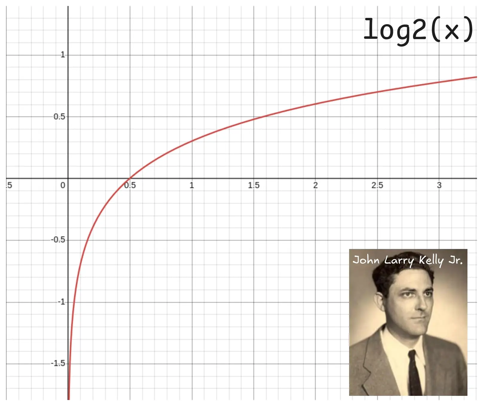
Diagram of a logarithmic function and Kelly himself.

The logarithm acts as a sort of model for losses compounding, because it tends to negative infinity very quickly for negative returns, penalizing losses and diminishes the effect large improbable wins have on the expected value.

Applying the Kelly Criterion to Ship Investor

To illustrate the power of the Kelly Criterion, we’ll be looking at the Ship Investor game that Entropic Thoughts designed. The player is a wealthy man in the 17th century, looking to invest in different shipments, trying to maximise his wealth. Every turn, four different investments are offered, for the same ship, but each having a different size.

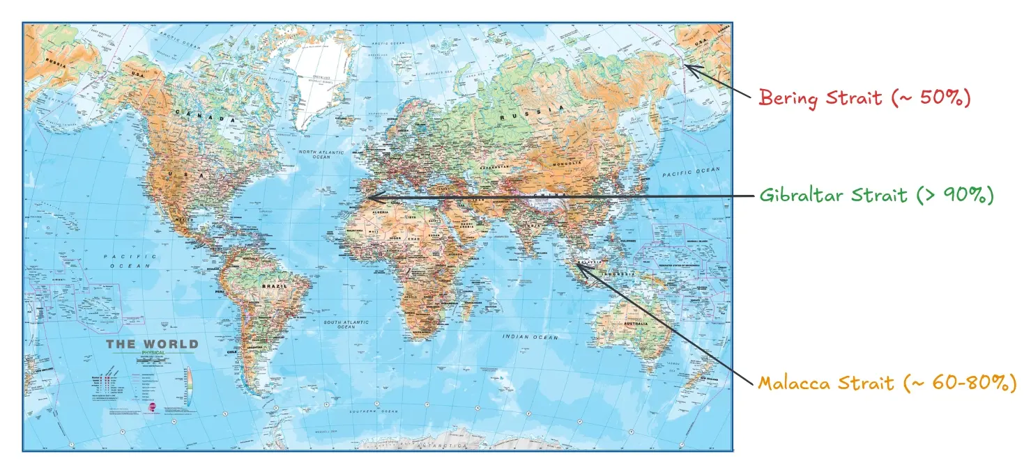
Your job is to determine the best investment, given the risks associated with the route the ships take. They can travel through the Gibraltar strait (very safe at over 90% success rate), the Malacca strait (between 60 and 80% of shipments pass) and the Bering strait (very unsafe, around 50% of ships pass).

I urge you to try it out before reading any further and to see if you would have had potential to be a wealthy magnate in bygone times.

World map showing the different straits and their safety ratings.

To succeed in the harsh business climate of past times and win the game, we always need to choose an investment that maximises our long-term wealth. Oh wait, isn’t that what the Kelly Criterion is for?

For situations where you either win a fraction of the investment or lose all of it (most gambling works like this), the Kelly Criterion takes a simplified form, that can be used to estimate the fraction of your wealth to invest.

f^* = p - \frac{(1 - p)}{B}

Where $f^*$ is the fraction of wealth to invest and $B$ is the proportion gained with a win (e.g. for a 1:1 odds bet $B = 1$ ).

Simulating different Agents in Ship Investor

To test this formula, I transcribed the ship investor game into a python script. I’ve created multiple investor types, each of which play with a certain agenda and mindset. Try it out and create your own agent: github.com/obrhubr/kelly-criterion-ship-investor.

Here is what 200 Kelly bettors wealth looks like, over a span of 500 turns.

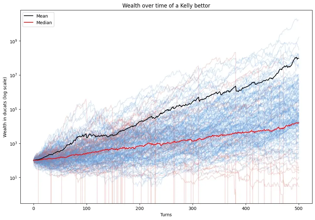
Graph showing the wealth over time of a large number of Kelly bettors.

On average, the bettors take a large profit, increasing their wealth from 100 ducats to over 100 million in 500 steps. The median wealth is also on a steady climb. But some unlucky investors take a large hit, because over 10k turns, even 1 in 10000 events happen and they lose everything.

This is why most people use fractional Kelly, choosing to invest only half or even a quarter of the Kelly bet to decrease risk even more.

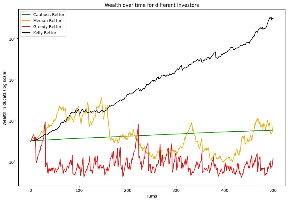
If we compare the Kelly bettors to other investment strategies, a cautious, median and greedy bettor, we can see why the Criterion is widely used. Even though in the short term, due to luck other strategies might outperform Kelly, it ends up on top - by a large margin - in the long term.

Different betting strategies compared to the Kelly bet.

Deriving the Gambling Formula

So how do we get from the general rule of maximising logarithmic wealth to the very specific gambling formula for sizing your bets?

First, we express your wealth at step $n$ . $W$ and $L$ are the number of wins and losses.

W_n = (f B + 1)^W \cdot (1 - f)^L

We can also express $W$ and $L$ with respect to $p$ and $n$ .

\begin{align} p &= \frac{W}{n} \\\ q &= \frac{L}{n} = 1 - p \end{align}

We can then express $W_n$ with respect to $n$ and $p$ .

W_n = (fB + 1)^{np} \cdot (1 - f)^{nq}

Now, we apply the Kelly Criterion, and get the growth rate $G$ .

\begin{align} G &= \lim_{n \to +\infty} \frac{1}{n} (\log(W_n)) \\\ &= \lim_{n \to +\infty} p \cdot \log(fB + 1) + q \log(1 - f) \end{align}

To find the optimal fraction to invest - the Kelly bet - we want to find the fraction for which $G$ is at it’s maximum - where the growth rate is the highest. By solving $\frac{\text{d}}{\text{d} f}G = 0$ , we find the inflection point, the highest point on a concave curve, and thus the Kelly bet.

The graph shows the growth rate as a function of the invested fraction. You can try to play around with the above function on Desmos for different probabilities and returns.

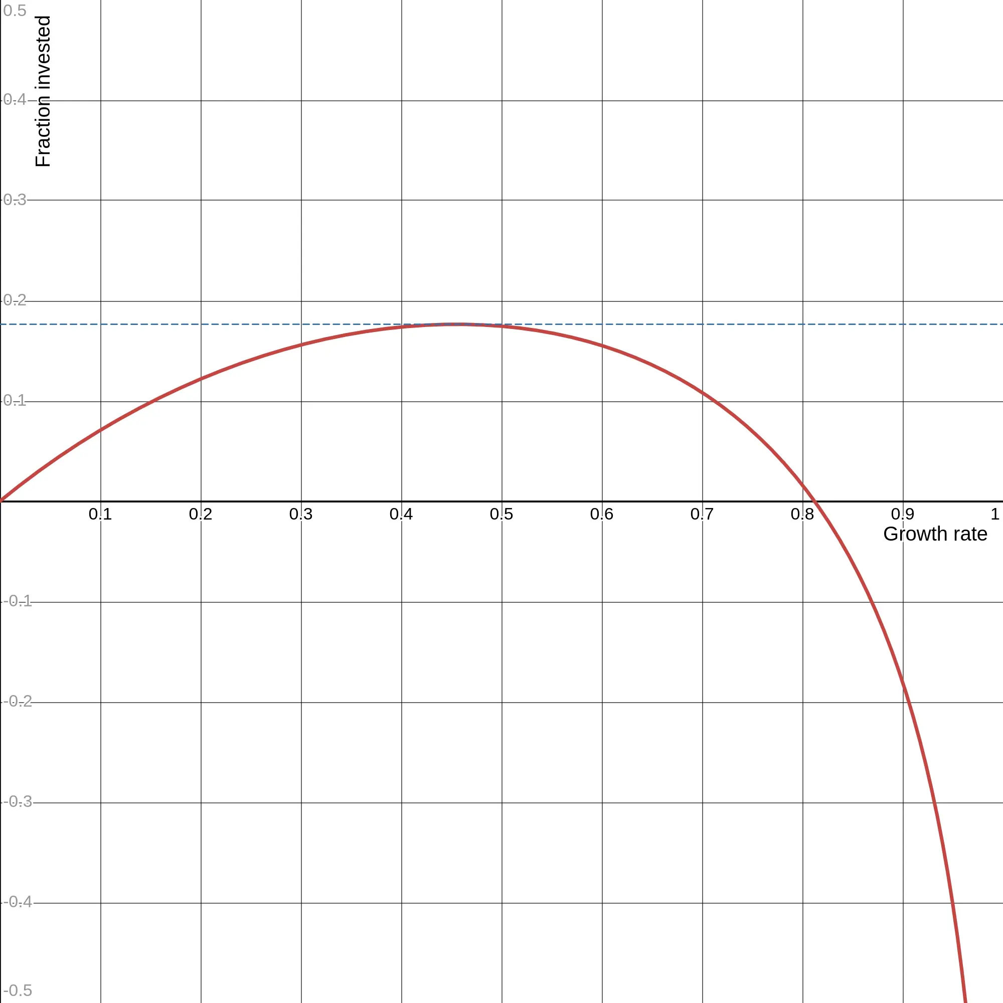
$Graphing the growth rate against the fraction of wealth invested.$

\begin{align} \frac{\text{d}}{\text{d} f}G = 0 \\\ \frac{\text{d}}{\text{d} f} \cdot p \log(fB + 1) + \frac{\text{d}}{\text{d} f} \cdot q \log(1 - f) = 0\end{align}

And by replacing $q = 1 - p$ this can be simplified to the following.

\begin{align} \frac{pB}{(fB + 1)} &= \frac{q}{1 - f} \\\ f(1 - p + p) &= p - \frac{(1 - p)}{B}\end{align}

Which gives us the gambling formula.

f = p - \frac{1 - p}{B}

If you want a better, more detailed explanation of the maths, I would recommend this great post on the topic.

Applying the Kelly Criterion to Blackjack

Kelly’s strategy clearly works in a simple scenario with a binary outcome: you either get the shipment to the port intact - or it sinks. But it can also be used to size bets in more complex games, such as Blackjack.

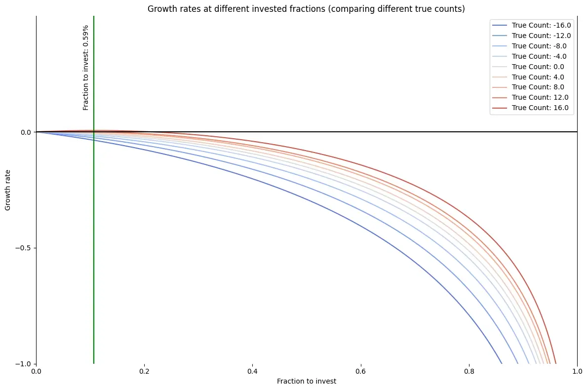
Instead of only even-odds, the game also offers 3:2 odds for a blackjack, a sum of 21 in the first two cards. But Blackjack’s win probabilities vary wildly, depending on which cards were drawn from the deck already. This is quantized in what’s called the true count. Since aces and tens are more favourable for the player (drawing an ace and a ten makes 21), a deck containing more of these cards increases the probability of a 3:2 payout - which increases the fraction the player should invest.

I wrote a simulation that plays about ten thousand hands of blackjack for each true count, determining the probabilities of the different payouts. You can try and play around with the code for Blackjack, it’s hosted on GitHub.

With this data, we can then determine the growth rate for the fraction invested as a line on the graph below. The Kelly Bet is the fraction with the highest growth rate, marked with the green line here, for a true count of +16 (which is very rare) at 0.59%. For negative counts, you shouldn’t bet at all according to Kelly.

Graph showing growth rates for different true counts in Blackjack. Playing with one deck, reshuffling at 25%. Dealer stands on soft 17, no doubling.

In practice, this means that professional gamblers counting cards are betting more on tables with high counts and the allowed minimum at tables with a low count in order to maximise growth.

But because it’s such as slight edge, you would have to play a lot to win a significant amount. If you’re interested in watching professional gamblers exploiting this edge, see Steven Bridges on Nebula or YouTube.

Calculating Blackjack’s growth rate

To calculate the growth rate in Blackjack (assuming we know the different probabilities) we have to determine the limit of the logarithm of the expected wealth for the number of hands played approaching infinity, as done above with the ship investor situation.

Instead of two, we now have three possible outcomes: the player wins with 21 and gets 3:2 odds, the player wins and gets 1:1 odds or he loses his investment.

\begin{align} G &= p_{3:2} \cdot \log(1 + 1.5f) + p_{1:1} \log(1 + f) + p_{0} \log(1 - f) \end{align}

Why isn’t everyone rich thanks to the Kelly Criterion?

If this magic formula is able to optimise growth rate that effectively, why isn’t everyone rich already? Clearly not even Kelly can turn a losing bet into profit.

The Criterion is very sensitive to change in the probabilities used, which have to be exact in order for the invested fraction to be correct. To hedge against this, a fractional Kelly bet is often used. This means that only 50% or 25% of the calculated fraction is invested. This is a valid strategy because - as you might already have observed - the growth rate is never negative for a fraction between 0 and the Kelly bet. Thus investing less will never lead to losing money.