If you have ever been skiing you surely searched the app store for an app that records your day on the slope. There are however lots of choices for apps logging the route, top speeds and the total distance travelled. How do they actually work?
The brief and disappointing answer is that GPS provides altitude, speed and location data, which makes it trivial to deduct if you are sitting on a lift (moving up) or skiing (moving down).
However, this total reliance on GPS surprised me, because most modern phones have built-in sensors such as accelerometers and gyrometers, that can be used to capture real-time data. Shouldn’t they be capable of more accurately delivering information about top speed or distance travelled? But most importantly, how could GPS be better at differentiating between slopes and lifts?
As such, I set out to develop my own ski tracking app, that uses only sensor data to distinguish skiing or riding the lift.
Collecting the Data
To collect the data needed to conduct this experiment, I relied on an application called Sensor Logger by Kelvin Choi. It provides a great interface and enables exporting to formats such as CSV.
Next, I set out to do the most important (and fun) part of this project, the actual skiing. I activated the sensor logger app multiple times, tracking sessions between one and three hours in Kitzbühel, Austria.
The data I collected was accelerometer, gyrometer and GPS information. The GPS would serve as ground truth later, to label my training dataset.
Labelling and Reshaping the Data
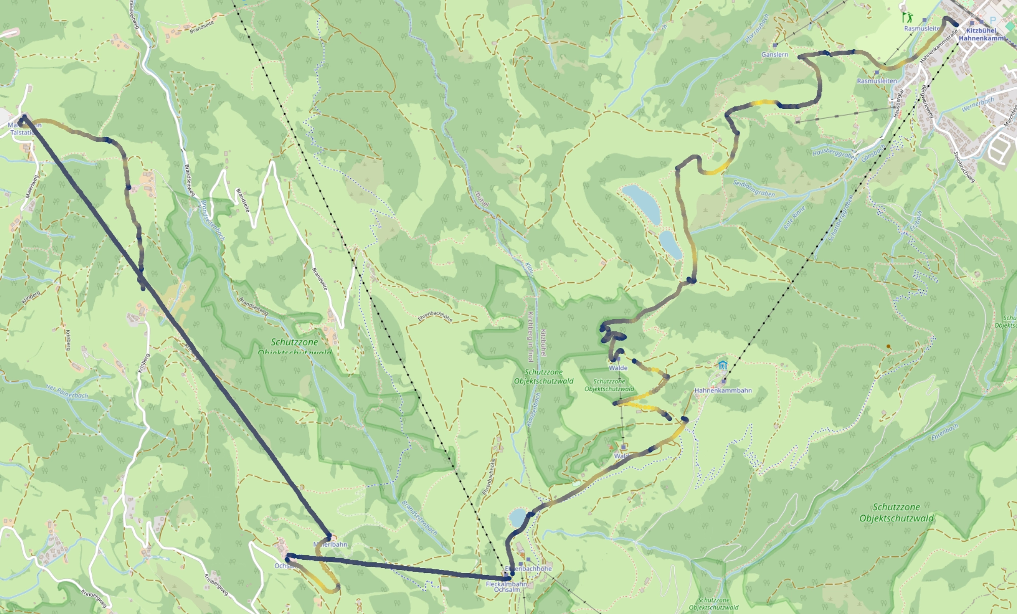
To label the data I utilized Python to visualize each GPS coordinate point on a map. By examining the shape of my tracks, I gauged whether a particular data point indicated sitting on a lift or skiing down a slope. I was further helped by the colouring of the tracks, corresponding to the speed (the lighter the colour, the faster).
As you can immediately tell, long straight lines at constant speed clearly match the pattern of a lift, narrow winding tracks match the twists and turns of the slope following the natural gradient of the mountain.
{
	"train_labels": [
		("2023-12-29 08:45:00.215311000", "lift"),
		("2023-12-29 09:00:06.228473000", "slope"),
		("2023-12-29 09:02:50.231005000", "lift"),
		....
		("2023-12-29 11:46:24.392286000", "slope")
	]
}
To feed this data to a machine learning model of our choice however we would have to wrestle it into shape first. The data should take the form of a timeseries. In practical terms, this involved concatenating a specific number of consecutive data points (e.g. 100 data points, roughly corresponding to 1 second) for each desired channel or feature (for example gyro_x, gyro_y and gyro_z) to a single row in our training dataset.
The label, distinguishing between slope and lift, can be either 0 or 1 making this a binary classification problem.
Creating the dataset
Building our dataset requires two important decisions to be made: First, how many data points should we feed the model with each training example? And second, which features should we keep?
The data logging app on my phone sampled the sensors at a very high frequency, a hundred data points correspond to only about a second. Therefore, I at first selected 100 data points and 6 features as a baseline, those being gyro_x, gyro_y, gyro_z, acce_x, acce_y, acce_z. I want to use a more scientific methodology to determine these values later, but this first choice proved sufficient for initial exploration.
This is what the data looks like in csv format. Notice that each feature (for example gyro_x here) actually corresponds to many columns, each for every data point sampled per row.
| gyro_x_0 | gyro_x_1 | gyro_x_2 | gyro_x_3 | gyro_x_4 | gyro_x_5 | gyro_x_6 | gyro_x_7 | gyro_x_8 | gyro_x_9 | … | acce_z_43 | acce_z_44 | acce_z_45 | acce_z_46 | acce_z_47 | acce_z_48 | acce_z_49 | longitude | latitude | label | |
|---|---|---|---|---|---|---|---|---|---|---|---|---|---|---|---|---|---|---|---|---|---|
| 0 | 0.111867 | 1.789682 | 1.142471 | 0.786387 | 0.430304 | 0.074220 | 0.705346 | 1.336471 | 1.967597 | 1.793500 | 1.619404 | … | -1.667821 | -2.287700 | -2.907579 | 0.661848 | 2.446561 | 4.231274 | 12.333252 | 47.43103 | slope |
| 1 | 1.867655 | 1.445307 | 0.794430 | 0.143553 | -0.507324 | -0.428675 | -0.350026 | -0.271377 | -0.382351 | -0.493325 | -0.604298 | … | -0.983435 | 0.024599 | 0.427315 | 0.628673 | 0.830031 | 1.521780 | 12.333252 | 47.43103 | slope |
| 2 | 2.526082 | -0.170839 | 0.262621 | 0.696081 | 0.037975 | -0.620130 | -1.278236 | -1.018363 | -0.758491 | -0.498619 | -0.582664 | … | -2.380495 | -1.199338 | -0.608760 | -0.018181 | 1.253950 | 1.890016 | 12.333252 | 47.43103 | slope |
| 3 | 0.099905 | -0.666709 | -0.750753 | -0.052178 | 0.646397 | 1.344973 | 0.824566 | 0.304160 | -0.216246 | -0.215075 | -0.213905 | … | -2.138179 | -2.576623 | -3.015066 | -1.555420 | -0.825596 | -0.095773 | 12.333252 | 47.43103 | slope |
| 4 | -1.737765 | -0.212734 | -0.098655 | -0.041615 | 0.015424 | 0.129503 | 0.359443 | 0.589383 | 0.819323 | 1.035926 | 1.252528 | … | -0.089555 | -0.217934 | -10.833972 | -16.141991 | -21.450010 | -8.308513 | 12.333252 | 47.43103 | slope |
Modeling: starting simple
Most often, the simplest solutions work best and as such I wanted to give a simple network a shot at classifying our data first. My initial attempt at building a simple neural network looked like this in tensorflow:
# Create a simple perceptron with 3 hidden layers
model = tf.keras.models.Sequential([
		tf.keras.layers.Dense(256, activation='relu', input_dim=channels*length),
		tf.keras.layers.Dense(128, activation='relu'),
		tf.keras.layers.Dense(64, activation='relu'),
		tf.keras.layers.Dense(num_classes, activation='sigmoid')
])

model.compile(loss=tf.keras.losses.BinaryCrossentropy(),
		optimizer=tf.keras.optimizers.Adam(),
		metrics=['accuracy']
)
The first results, after training the model for 50 iterations, were thoroughly disappointing, with the model achieving only 0.618 accuracy on our validation dataset. This corresponds to 61.8%, only marginally better than guessing (which would be 50%).
I could see the validation_accuracy jumping around during training while the accuracy began approaching 1.00 which suggests overfitting.
This table shows the accuracy of the model corresponding to the different numbers of datapoints provided as the input:
| type | datapoints | accuracy |
|---|---|---|
| simple | 50.0 | 0.597457 |
| simple | 100.0 | 0.618493 |
| simple | 200.0 | 0.602071 |
| simple | 300.0 | 0.606137 |
| simple | 400.0 | 0.598302 |
| simple | 500.0 | 0.599454 |
Before jumping to conclusions however, I wanted to try a convolutional model, more apt for complex timeseries problems.
Modeling: convolutional models
One of the most popular Python libraries for building machine learning models is Keras. It’s official documentation suggests using convolutional models to classify timeseries.
But what is a convolutional neural network? A convolution is a special operation on data that reduces it’s dimensionality (which means size in this context) by applying a sort of mask (called a kernel) to produce new results (called filters). These filters often show patterns more clearly, making this type of network ideal for pattern recognition. 3Blue1Brown created a great explanation video in case you want to learn more.
The documentation provides an example model architecture:
# Create a convolutional model with 3 convolution steps

input_layer = keras.layers.Input(input_shape)

conv1 = keras.layers.Conv1D(filters=64, kernel_size=6, padding="same")(input_layer)
conv1 = keras.layers.BatchNormalization()(conv1)
conv1 = keras.layers.ReLU()(conv1)

conv2 = keras.layers.Conv1D(filters=64, kernel_size=6, padding="same")(conv1)
conv2 = keras.layers.BatchNormalization()(conv2)
conv2 = keras.layers.ReLU()(conv2)

conv3 = keras.layers.Conv1D(filters=64, kernel_size=6, padding="same")(conv2)
conv3 = keras.layers.BatchNormalization()(conv3)
conv3 = keras.layers.ReLU()(conv3)

gap = keras.layers.GlobalAveragePooling1D()(conv3)

output_layer = keras.layers.Dense(num_classes, activation="sigmoid")(gap)

model = keras.models.Model(inputs=input_layer, outputs=output_layer)
The best results with the convolutional network were achieved with 400 datapoints, four times more than what the simple perceptron performed best with. This trade-off improved performance by 5%, which might make it worth it.
| type | datapoints | accuracy |
|---|---|---|
| conv | 50.0 | 0.566254 |
| conv | 100.0 | 0.605583 |
| conv | 200.0 | 0.631030 |
| conv | 300.0 | 0.646547 |
| conv | 400.0 | 0.663158 |
| conv | 500.0 | 0.644149 |
But Wait, Let’s Look at the Predictions
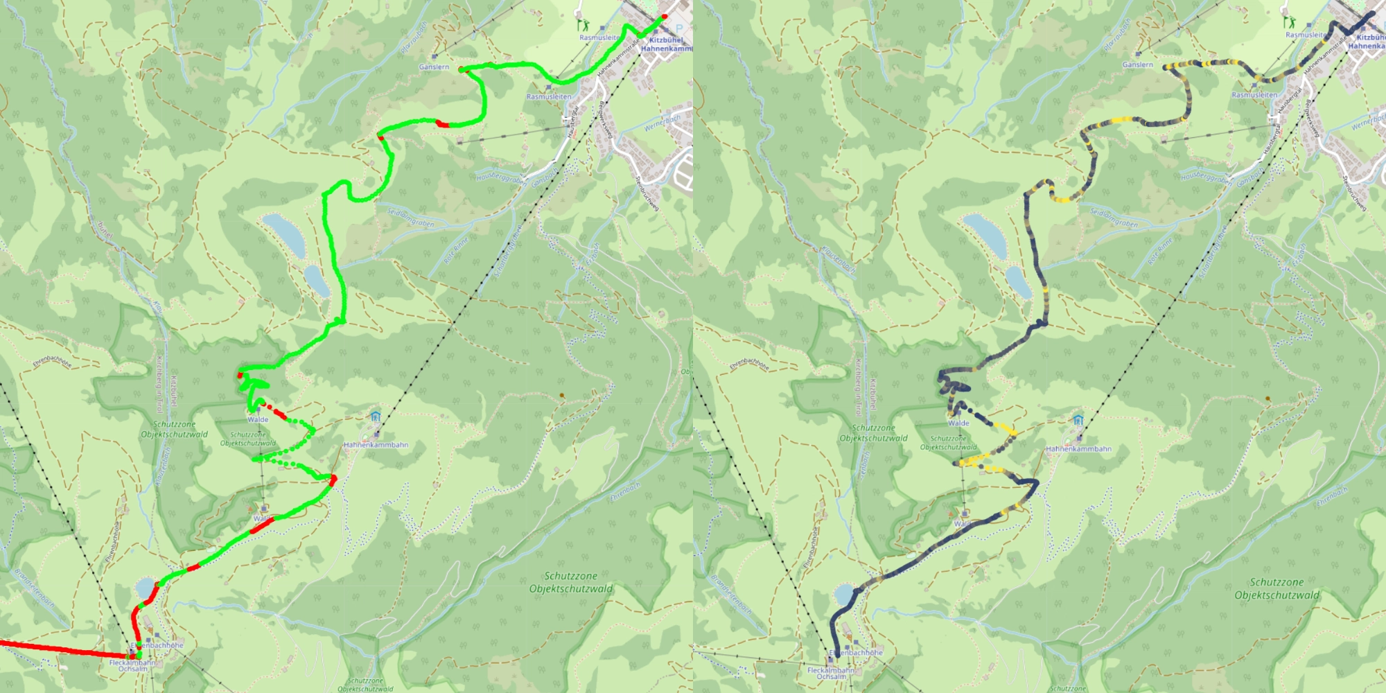
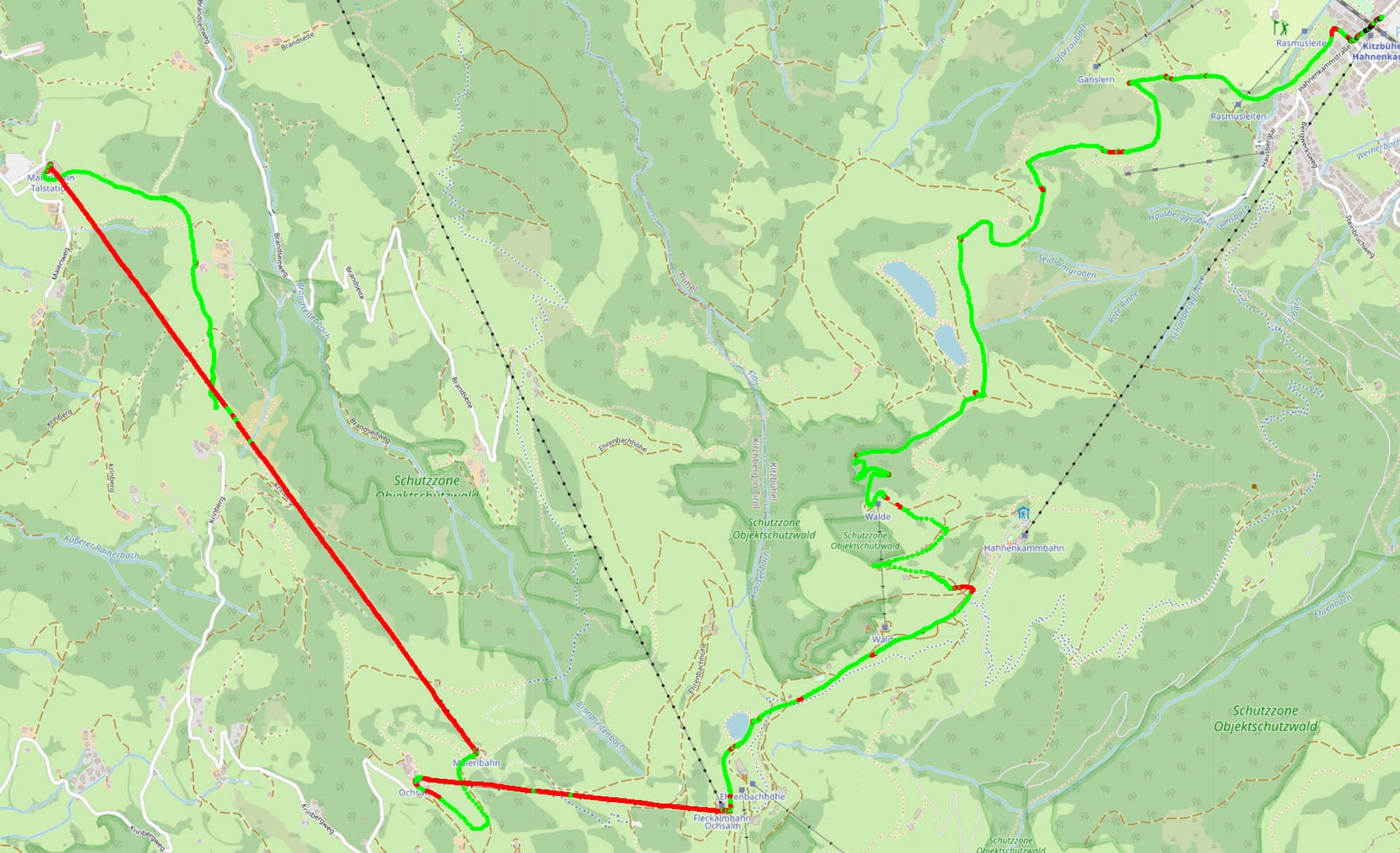
To get a feeling for where our model was hitting it’s limits, I wanted to visualize the location data and the corresponding prediction that the model made. A red point corresponds to what the model predicts is lift, a green point corresponds to slope.
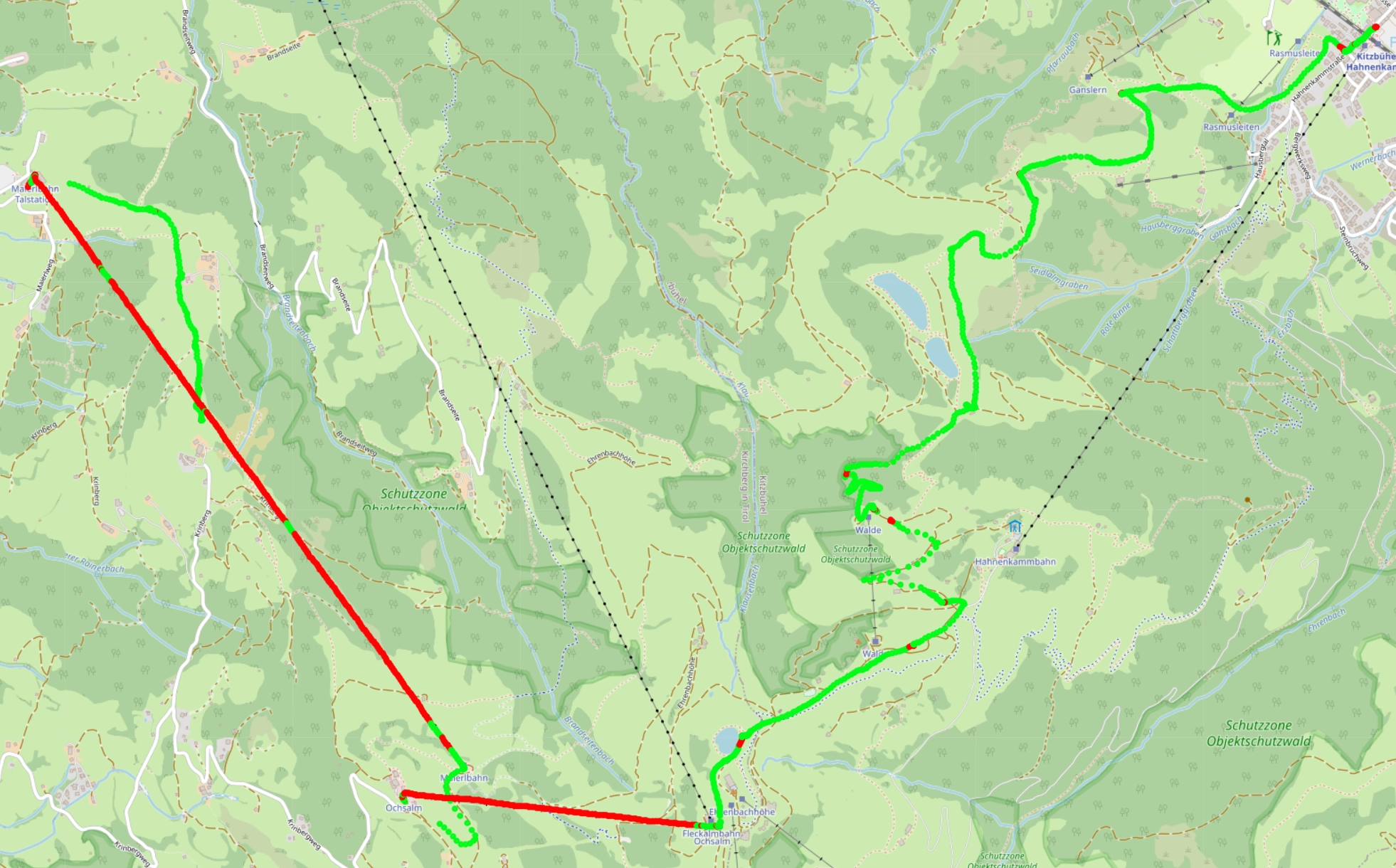
Now there are two interesting things that we can gleam from this map.
-
On the big lift, connecting the two mountain peaks Hahnenkamm and Jochberg (the large red line on the left side of the map), we see multiple, equidistant green sections, meaning the model interpreted these sections as slope. Why could that be? My theory is that these sections correspond to the time where the gondola travelled over the supporting pillars, which usually shakes it quite a bit. This could have been enough to trigger the model to mistake it as slope.
-
Then there are also red lift sections dotted all over my runs, especially on the final run into the valley (right side). These could correspond to times where I stood still on the slope, waiting for my friends to catch up or the slope to clear up. If we cross reference this map with the first one, these sections all have slow speeds in common.
Instead of saying I have a model with only slightly better than random accuracy, I prefer to say that my model is better at labelling my data than me. You could make the case that you would actually want the model to classify sections where I stood still as lift (or “not skiing”), depending on the use case.
In case you want continuous sections of alternating slope and lift, you could use post-processing to remove these small imperfections.
However, I still wanted to try to get the model to improve it’s accuracy, hoping that more training and optimization might make it possible to distinguish standing still from sitting on a lift.
Let’s Improve the Model
My first idea was to look at the data collected again. The exact features I had access to were:
df = df[["z","y","x","qz","qy","qx","qw","roll","pitch","yaw","z_gyro","y_gyro","x_gyro", "label"]]
The qz, qy, qx and qw correspond to quaternion rotation data, which is a special way to represent rotation in space with the use of four real numbers, the rest of the column names being self-explanatory.
I used sklearn to rank the different features based on univariate statistical tests with SelectKBest. This resulted in the following ranking:
| rank | 1 | 2 | 3 | 4 | 5 | 6 | 7 | 8 | 9 | 10 | 11 | 12 |
|---|---|---|---|---|---|---|---|---|---|---|---|---|
| feature | pitch | qy | qx | qz | qw | y | roll | x_gyro | yaw | z_gyro | x | z |
To try to improve the model’s performance, I tried using the top 6 features (y, qz, qy, qx, qw and pitch), instead of choosing x, y, z, gyro_x, gyro_y and gyro_z arbitrarily.
I trained the same convolutional model on data of the same length (400 datapoints) with the same number of channels (6). The results of this experiment were as follows:
| features | model | epochs | accuracy |
|---|---|---|---|
x, y, z, gyro_x, gyro_y, gyro_z
|
conv | 60 | 0.663158 |
y, qz, qy, qx, qw, pitch
|
conv | 60 | 0.693548 |
An improvement of 0.03 in accuracy, just from changing the features used, nice!
Let’s Tune the Model Parameters
But we can try even more tricks to improve model performance and edge out the last few percent.
The keras_tuner python library provides a simple interface to do hyperparameter tuning with keras models. But what does this actually mean? When creating a model, there are a few choices we have to make, for example the amount of hidden layers, the neurons in each layer and for convolutional networks, the size of the kernel and filters. More neurons and layers can mean more performance in some cases, such as deep learning, but not always.
These hyperparameters are usually first set by guessing and intuition, but often trying out many different combinations can improve performance. Instead of doing this manually, keras_tuner allows us to set ranges for each of the parameters and it tries out all different combinations automatically, keeping track of the best ones.
# Defining the first convolutional layer of our model
conv1 = keras.layers.Conv1D(
	# The number of filters can vary between 32-128
	filters=hp.Int("filters", min_value=32, max_value=128, step=32),
	# The kernel size between 4-10
	kernel_size=hp.Int("kernel_size", min_value=4, max_value=10, step=2),
	padding="same"
)(input_layer)
The tuner found that the best-performing hyperparameters were {"filters": 96, "kernel_size": 6}, resulting in an accuracy of 0.73089, another 4% improvement.
The Final Predictions
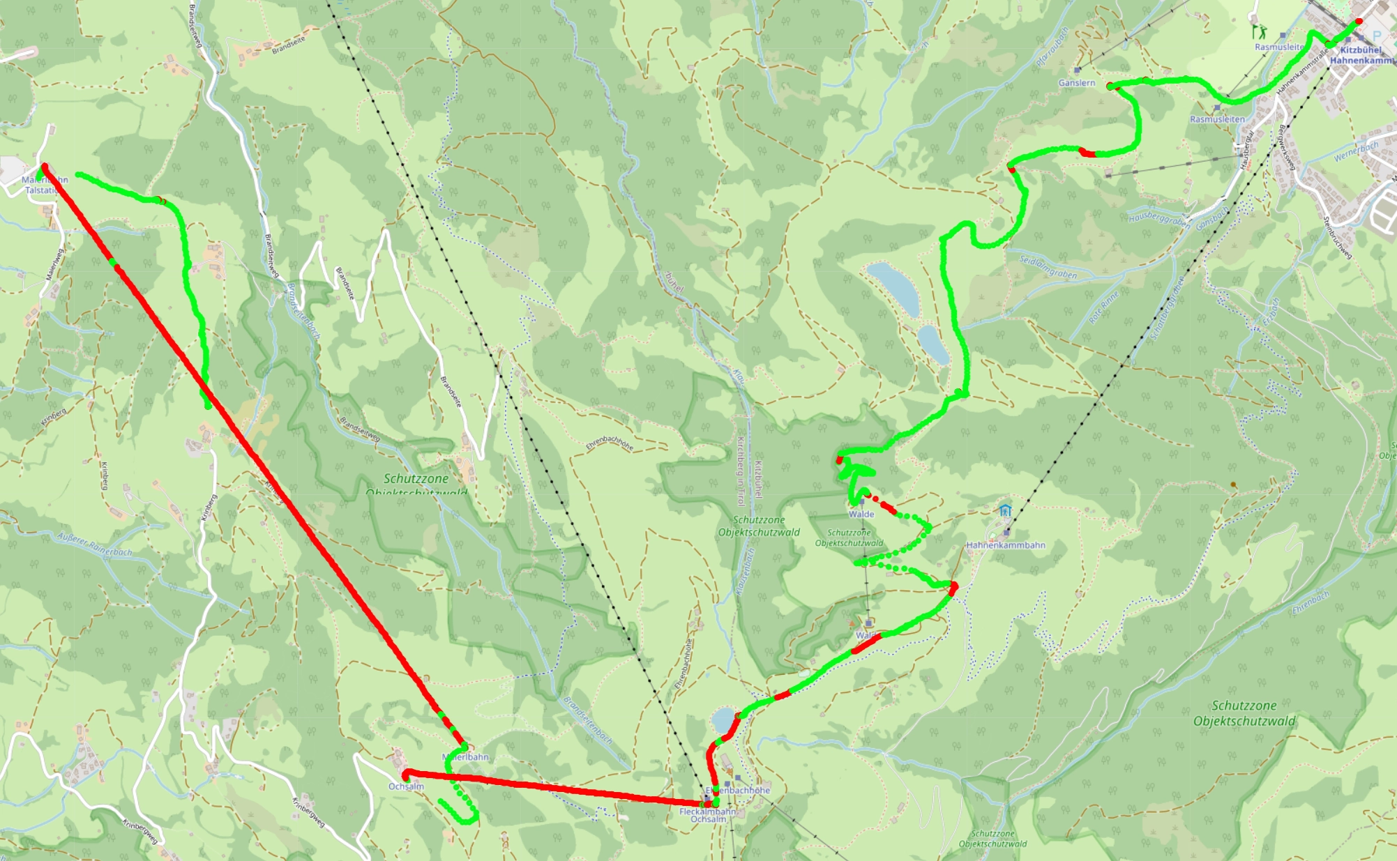
Here is what the predictions of this last and best model look like. Still not perfect right? You might even say worse than before. But what has improved a lot is the recall for the lift sections, which is mostly correctly labelled. But now it incorrectly labels some slope sections as lift. Let’s look at a few more maps to understand what is going on with the slope sections though.
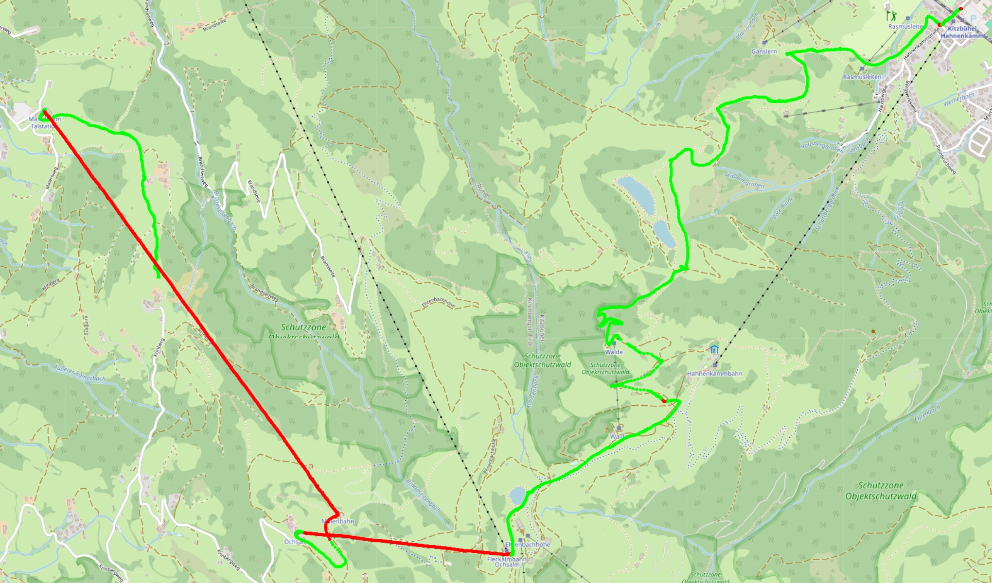
The right map shows the predictions of the model, the left map shows the speed (lighter means faster).
Now, if you look at the incorrectly predicted sections (red sections), the colour on the right map is dark, meaning the speed was relatively slow and more important, the speed is very constant over these sections.
Why is that important? Because the accelerometer can only pick up changes in speed. The incorrectly identified sections are long, straight lines, without much change in speed or just sections where I stood still. Sounds familiar? Because this description could also match what happens on a lift. This explains the model’s confusion.
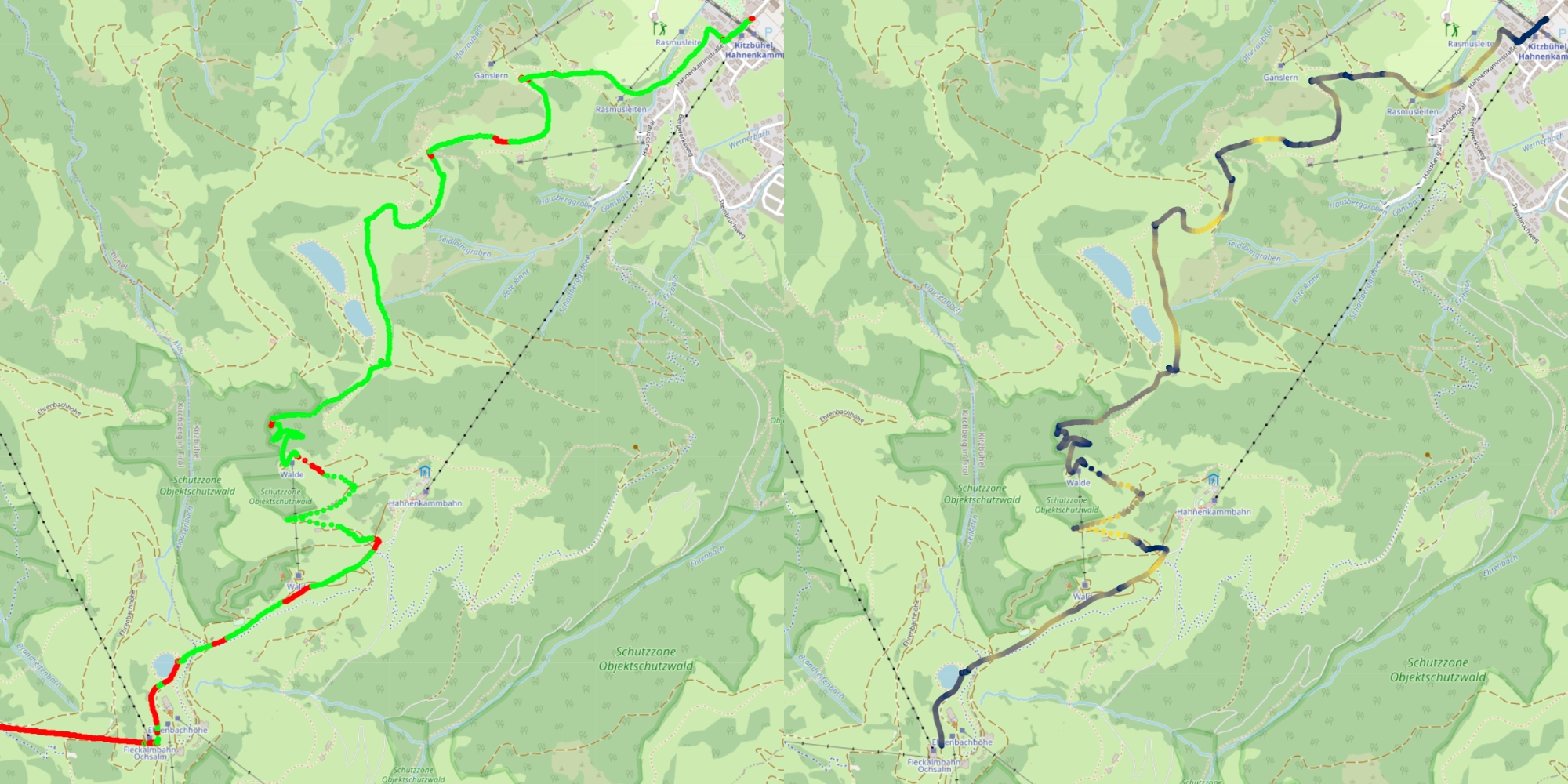
If we look at this map, which shows the vertical speed you can see that the incorrectly labelled sections are mostly straight horizontal sections, because the colour is dark (meaning low rate of change of altitude). This further corroborates the hypothesis above.
Let’s look at the actual data for these few sections now. Each of these plots correspond to 10s of data, one of them was on a lift, the other on one of the long straight skiing sections. Try to guess which is which:
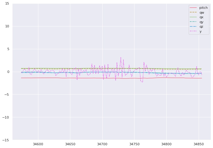
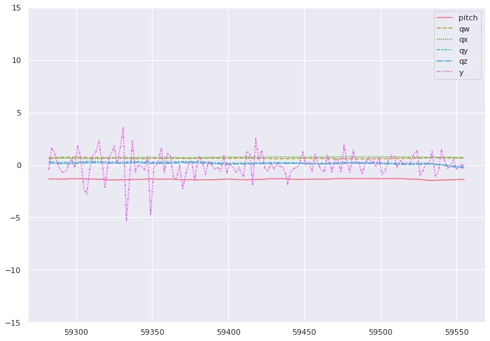
If you guessed that the first graph corresponds to the section travelled on the lift, you guessed correctly and can now officially claim that you are more proficient at pattern-matching than AI thanks to millions of years of evolution.
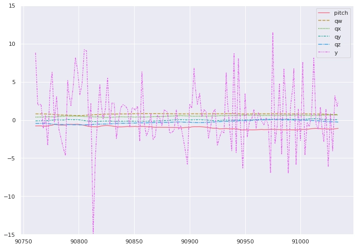
Just for comparison, this is what actual skiing looks like:
What Now?
Currently, the model is not very useful: you don’t want to have to bust out your laptop on the slopes and run a Jupyter Notebook, just to get an imperfect estimation of your time spent skiing.
However, the model could be exported in TFLite format, making it suitable for mobile devices. It could be integrated an app and be the world’s most battery intensive ski tracker. How do the real ski tracking apps do it: let’s try to recreate their algorithms.
Can I do better with GPS Data?
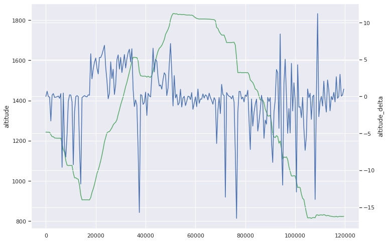
This graph shows the altitude and altitude_delta over time. A negative altitude delta means going down, a positive delta means going up. One interesting thing is that on lift sections, your are not guaranteed to only be going up, as pillars and straighter sections could temporarily slow ascent. Another anomaly are the very high spikes in altitude during the last descent, which could correspond to sections where the slope is going upwards for a very short time or jumps.
If we use the very simple heuristic of going up means lift and down means slope we get an imperfect result, not too dissimilar to what our model outputs.
To improve this, we can aggregate a few thousand datapoints together take the average over those. We now get nearly perfect labelling at a fraction of the cost of running a machine learning model. It also only took me 15 minutes to figure this out, instead of the weeks spent optimising the model.
But where would be the fun in that?